对光斑点阵进行提取代码与解释

光斑分割

发布日期: 2022-04-15

更新日期: 2022-10-29

文章字数: 1.1k

阅读时长: 5 分

阅读次数:

1.代码

代码先放这

function  shwfs_make_coarse_grid(img)
sh_flat = img;          %加载成像点图
% tunable parameters                 %加载需要使用的参数
thresh = 0.08; %二值化用阈值 0.08例子代码
npixsmall = 8;      %可以认为是噪声光斑的尺寸阈值    
strel_rad = 8;      %粗网格半径
radius =10;%粗网格半径传递于radius=16
%% thresh = graythresh(sh_flat);
%这里的算法可以改进为自适应阈值，使用灰度统计后进行
    bw = im2bw(sh_flat, thresh);             %不减背景图像后二值，阈值0.08
% 获取二值图像并显示
sfigure(3);
imshow(bw);
title('binary image');
%% remove small objects
bw = bwareaopen(bw, npixsmall);%matlab自带函数bwareaopen()，定义尺寸后自动消除小于此尺寸物体，注意输入要为二值
% sfigure(4);
% imshow(bw);
% title('remove small objects 1');
%% remove edges
% strel形态学处理函数
% 创建圆盘半径8
se = strel('disk',strel_rad);
bw = imclose(bw, se);%闭运算
% sfigure(5);
% imshow(bw);
% title('remove small objects 2');
%%
cc = bwconncomp(bw, 4);%找连通分量
s = regionprops(cc, 'Centroid');%检测图像区域的属性，寻找连通分量的质心
nspots = length(s);%计数，质心个数
hold on;
for k = 1:nspots
    c = s(k).Centroid;    %获取质心坐标后绘制源泉
    plot(c(1), c(2), 'ro');
end
squaregrid = zeros(nspots, 4);%这里获取一个质心点数量*4的0矩阵
sfigure(6);
imshow(sh_flat);
hold on;
for k = 1:nspots
    c = s(k).Centroid;
    plot(c(1), c(2), 'ro');%再画一遍看看效果
end
%下面的for函数定位画框，顺带画个框
for k=1:nspots
    c = s(k).Centroid;
    c = round(c);%取整
    minx = c(1) - radius;
    maxx = c(1) + radius;
    miny = c(2) - radius;
    maxy = c(2) + radius;
    box = [minx, maxx, miny, maxy];%为一个20*20的框
    squaregrid(k, :) = box;%每一行为一个矩形
    sfigure(6);
    hold on;
    rectangle('Position', [minx, miny, maxx-minx+1, maxy-miny+1], ...
        'LineWidth', 2, 'EdgeColor', 'b');%绘制矩形框
    sfigure(15);%函数用于重置
    % image is height times width!
    box(3)
    box(4)
    box(1)
    box(2)
    subsfigure = sh_flat(box(3):box(4), box(1):box(2));
    imshow(subsfigure);%切割出每个小块
    pause(0.01);
end
 nspots
% [minx, miny, maxx-minx+1, maxy-miny+1]
% image plot coords
squaregrid%存储点图坐标点进入结构体
end

2.代码分段讲解

光斑点阵图

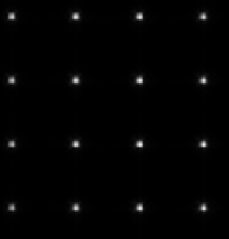
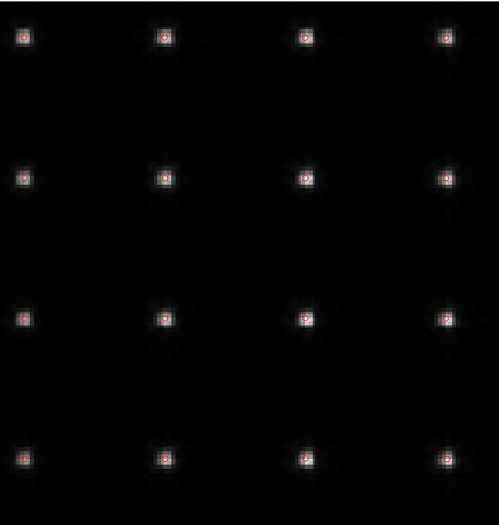
这图先拿来讲解，顺带讲讲开运算闭运算连通分量的数学原理

sh_flat = img;           %加载上面那个图
%% tunable parameters                 %加载需要使用的参数
thresh = 0.08;      %二值化用阈值 0.08例子代码
npixsmall = 8;      %可以认为是噪声光斑的尺寸阈值    
strel_rad = 8;      %粗网格半径
radius =10;%粗网格半径传递于radius=16
% 记住这些参数，都有用
%% thresh = graythresh(sh_flat);

%这里的算法可以改进为自适应阈值，使用灰度统计后进行
bw = im2bw(sh_flat, thresh);             %不减背景图像后二值，阈值0.08
% 获取二值图像并显示
sfigure(3);
imshow(bw);
title('binary image');

计算完之后的二值图长下面那个样子：

我是binary

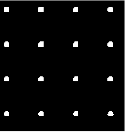
bw = bwareaopen(bw, npixsmall);%matlab自带函数bwareaopen()，定义尺寸后自动消除小于此尺寸物体，注意输入要为二值,这下就能知道npixsmall的用途了

这里去除掉一部分过于小的点，能够去除一部分噪声，但是也有可能去除掉一些微弱的信号

%% remove edges
% strel形态学处理函数
% 创建圆盘半径8
se = strel('disk',strel_rad); %创建一个指定半径strel_rad的平面圆盘形的结构元素
bw = imclose(bw, se);%闭运算，使用se对bw进行腐蚀后，再用se进行膨胀后结果
 sfigure(5);
 imshow(bw);
 title('remove small objects 2');
%%
cc = bwconncomp(bw, 4);%找连通分量
s = regionprops(cc, 'Centroid');%检测图像区域的属性，寻找连通分量的质心
nspots = length(s);%计数，质心个数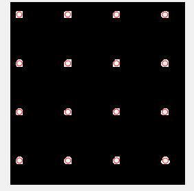

直接获取质心

for k=1:nspots
    c = s(k).Centroid;
    c = round(c);%取整
    minx = c(1) - radius;
    maxx = c(1) + radius;
    miny = c(2) - radius;
    maxy = c(2) + radius;
    box = [minx, maxx, miny, maxy];%为一个20*20的框
    squaregrid(k, :) = box;%每一行为一个矩形
    sfigure(6);
    hold on;
    rectangle('Position', [minx, miny, maxx-minx+1, maxy-miny+1], ...
        'LineWidth', 2, 'EdgeColor', 'b');%绘制矩形框
    sfigure(15);%函数用于重置
    % image is height times width!
    box(3)
    box(4)
    box(1)
    box(2)
    subsfigure = sh_flat(box(3):box(4), box(1):box(2));
    imshow(subsfigure);%切割出每个小块
    pause(0.01);
end

对原图进行分割，按照联通分量确定的质心

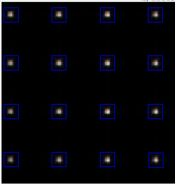
注意这个输出

下面是矩阵框的x方向像素范围和y方向像素范围的偏移由于闭运算被消减了。

4 24 9 29
4 24 79 99
4 24 150 170
4 24 220 240
74 94 9 29
74 94 79 99
74 94 150 170
74 94 220 240
145 165 9 29
145 165 79 99
145 165 150 170
145 165 220 240
215 235 9 29
215 235 79 99
215 235 150 170
216 236 221 241